How I Triaged a BigQuery Cost Spike at a Regional Grocery Chain — And the Two Problems Hiding in…
How I Triaged a BigQuery Cost Spike at a Regional Grocery Chain — And the Two Problems Hiding in the Query Patterns
Tags: BigQuery, Data Engineering, FinOps, Cloud Cost Optimization, SQL, GCP, Retail Analytics
If you run BigQuery for a retail operation at scale, your costs have probably crept up without an obvious explanation. I recently triaged a regional grocery chain where BigQuery spend had jumped 55% in just ten weeks. The platform team sorted jobs by bytes billed to find the culprit, but nothing stood out. That’s because the spike wasn’t caused by a single rogue query — it was driven by two structural query patterns and a hidden compliance data gap.
Start with the billing export shape, not the query list
Every cost investigation I’ve been called into starts the same wrong way: someone opens the BigQuery console, sorts jobs by bytes billed, and starts reading query text. That method finds the biggest query. It doesn’t find the real problem.
I always start with the billing export. Not to find the worst offender — to understand the shape of the cost growth.
SELECT
    DATE_TRUNC(usage_start_time, WEEK)                    AS week,
    project.id                                            AS project_id,
    SUM(cost)                                             AS total_cost_usd,
    SUM(IF(sku.description LIKE '%Queries%', cost, 0))    AS query_cost_usd,
    SUM(IF(sku.description LIKE '%Storage%', cost, 0))    AS storage_cost_usd
FROM `billing_export_dataset.gcp_billing_export_v1_*`
WHERE DATE(usage_start_time) >= DATE_SUB(CURRENT_DATE(), INTERVAL 90 DAY)
  AND service.description = 'BigQuery'
GROUP BY 1, 2
ORDER BY 1 DESC;
The breakdown was immediate: query cost had climbed linearly for ten weeks. Storage was flat. Streaming was flat. The transactions table wasn’t growing unusually fast. Queries were getting worse — either more of them, worse versions of existing ones, or both.
The next step was hitting INFORMATION_SCHEMA.JOBS_BY_PROJECT. Again, not to find the worst query, but to find the fleet. (Note: I'm using $6.25/TB for On-Demand pricing here to visualize cost, but even if you are on Enterprise Slot capacity, bytes scanned directly correlates to slot time and concurrency bottlenecks).
SELECT
    SUBSTR(query, 1, 150)                                   AS query_preview,
    user_email,
    COUNT(*)                                                AS executions_30d,
    ROUND(AVG(total_bytes_billed) / POW(1024, 3), 1)        AS avg_gb_billed,
    ROUND(SUM(total_bytes_billed) / POW(1024, 4) * 6.25, 2) AS total_cost_usd,
    COUNTIF(cache_hit) * 100.0 / COUNT(*)                   AS cache_hit_pct
FROM `region-us`.INFORMATION_SCHEMA.JOBS_BY_PROJECT
WHERE creation_time >= TIMESTAMP_SUB(CURRENT_TIMESTAMP(), INTERVAL 30 DAY)
  AND statement_type = 'SELECT'
  AND total_bytes_billed > 5 * POW(1024, 3) -- Lowered threshold to 5GB to catch the fleet
GROUP BY 1, 2
ORDER BY total_cost_usd DESC
LIMIT 50;
No single query was billing more than $40/day. The top offender was a demand forecasting query at $35/day — unremarkable for a platform. But there were eleven queries in that band, running between 6 and 180 times daily. No alert had fired because no individual query crossed anyone’s threshold. Together, though, they were billing nearly $240/day.
The cost spike wasn’t a bad query. It was a bad portfolio of queries.
The Patterns That Actually Mattered
I categorized the eleven queries by structural root cause rather than by dollar amount. Two distinct failure modes were driving the bulk of the spend.
1. The optimizer cannot push your filter through a window function
The demand forecasting workload was the largest single cost cluster. Six of the eleven queries shared a structural flaw. The retail analytics team had built a rolling 90-day sales velocity calculation to drive SKU replenishment triggers. The business logic was correct. The query structure was not.
The transactions table is partitioned by sale_date and holds about 280 million transaction baskets per year (roughly 4 billion nested line items).
BigQuery cannot push an outer query filter through a window function inside a CTE. The window function must evaluate all preceding rows to compute the rolling sum correctly. Therefore, BigQuery silently scans the entire transactions table (over 5 years of POS history) before the outer WHERE clause can discard anything.
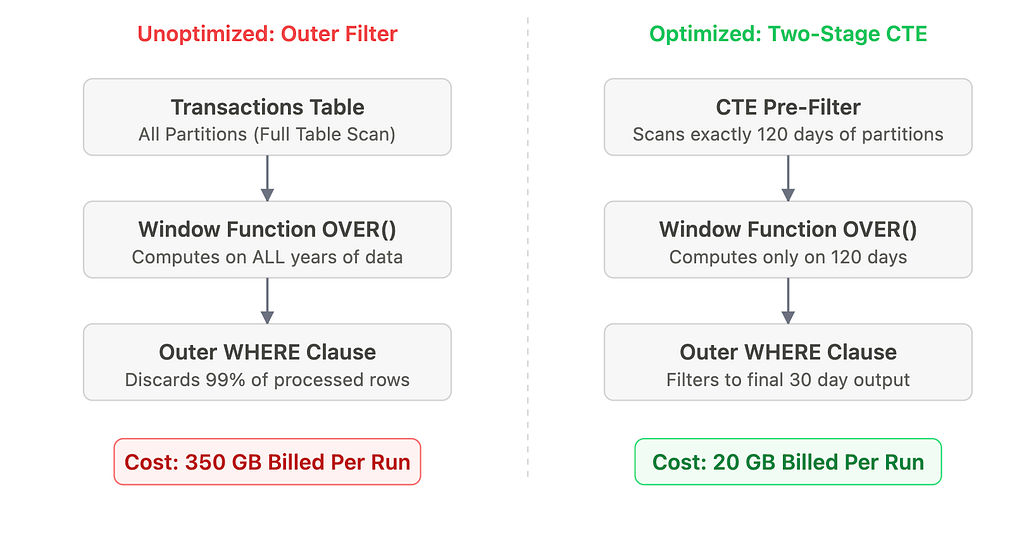
The fix is not “move the WHERE clause into the CTE.” That would break the rolling calculation, truncating the necessary lookback history. The correct fix is a two-stage base table that pre-filters to just wide enough of a window to give the window function the history it requires:
WITH base_transactions AS (
    -- Pre-filter to exactly window limit + lookback history
    SELECT t.sku_id, t.store_id, t.sale_date, t.quantity_sold
    FROM `analytics.transactions` t
    WHERE t.sale_date >= DATE_SUB(CURRENT_DATE(), INTERVAL 120 DAY)  -- 30d output + 90d lookback
),
sku_velocity AS (
    SELECT *,
        SUM(quantity_sold) OVER (
            PARTITION BY sku_id, store_id
            ORDER BY sale_date
            ROWS BETWEEN 89 PRECEDING AND CURRENT ROW
        ) AS rolling_90d_units
    FROM base_transactions
)
SELECT sku_id, store_id, AVG(rolling_90d_units) AS avg_velocity
FROM sku_velocity
WHERE sale_date >= DATE_SUB(CURRENT_DATE(), INTERVAL 30 DAY)
GROUP BY 1, 2;
Bytes billed dropped from 350 GB to 20 GB per execution. The “obvious” fix is wrong; the right fix requires sizing the base partition filter precisely to the algorithm’s requirements.
2. STRUCT column flattening is a silent scan amplifier
The basket analysis queries were the second major cost cluster. The loyalty analytics team runs promotional effectiveness reports for category managers.
The transactions table stores each purchase as a REPEATED STRUCT of line items: one record per transaction, with the basket contents embedded as an array, accounting for roughly 70% of the row width.
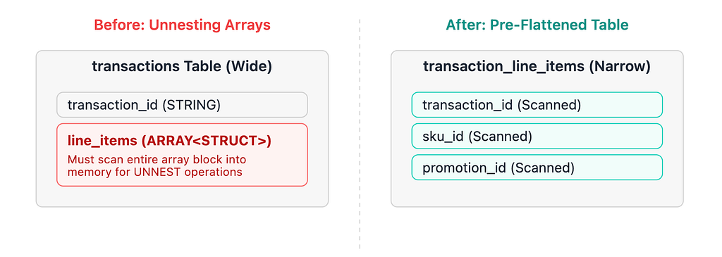
When you write a query utilizing CROSS JOIN UNNEST(t.line_items), BigQuery does dynamically prune the partition bytes. However, because BigQuery is columnar, it must scan the entire line_items column from every partitioned row into memory before the structural promotion_id filter can execute. For a standard supermarket averaging 15 items per basket, this is a massive penalty.
For high-frequency queries running daily, the path forward was a pre-flattened transaction_line_items table: one row per line item, partitioned by sale_date, clustered by promotion_id. The nightly flattening job is incredibly cheap. If your business users are running a dozen distinct promotional patterns against the same STRUCT column over and over, pre-flattening pays for itself in just days.
The PCI-DSS and GDPR Protocol You Cannot Ignore
This retailer processes payment data subject to PCI-DSS and handles loyalty data subject to local privacy regulations and GDPR. Both requirements drive logging patterns that have serious BigQuery cost implications. Their architectural gap? The application-level query audit table had accumulated 22 months of records but wasn’t partitioned by date because “audit logs aren’t operational data.”
Yes, they are. Partition your compliance audit tables exactly the same way you partition your fact tables.
Partitioning reduced the audit baseline cost by 65%. But “right-to-erasure” reporting requires scanning the full history for a given customer across years of data, meaning partition filters don’t fully solve the needle-in-a-haystack problem.
To bridge this, we implemented BigQuery Search Indexes (CREATE SEARCH INDEX idx_customer_id ON analytics.gdpr_query_audit_log(customer_id)). While BigQuery isn't an OLTP database, Search Indexes act like secondary indexes for high-frequency text lookups, preventing BigQuery from brute-force scanning gigabytes of log data every time it looks for a single shopper's lifetime footprint.
What The Architecture Looks Like After
Three months in, the settled numbers against their GCP invoice:
- Demand forecasting restructuring (window function pre-filtering): $3,400/month saved
- Basket analysis pre-flattening (top three queries): $1,850/month saved
- Audit log partitioning & search indexing: $240/month saved
Total reduction: $5,490/month (nearly $66,000 annualized). The combined BigQuery spend had peaked at $8,500/month and safely settled back down to about $3,000/month.
To ensure it stayed there, the platform team deployed preventative controls: require_partition_filter = TRUE on massive datasets, a CI-integrated dry-run check in dbt to reject queries exceeding a 50 GB scan limit, and a weekly scheduled audit script to flag zero-cache-hit query loops.
The pattern is the same everywhere
The cost wasn’t hiding; it was distributed. Neither problem surfaced in a simple top-N BigQuery console sort.
These patterns transcend BigQuery. In Snowflake, the exact same window function problem manifests as warehouse suspension failures (the rolling computation holds the warehouse active long past the auto-suspend timer). In Databricks, it shows up as brutal shuffle spill to disk.
The tools differ. The FinOps methodology — find the shape, identify the fleet, fix the structural root cause — doesn’t.
For those running retail analytics on BigQuery: how are you handling STRUCT and ARRAY columns in high-frequency analytical queries? Curious whether others have moved entirely to pre-flattened tables or found ways to make UNNEST-heavy patterns native and cost-effective.